
Xây dựng bộ phân loại VGG16 với Tensorflow Keras và áp dụng phân loại chó mèo

Dù Tensorflow Keras đã hỗ trợ VGG16, ở bài viết này, chúng ta vẫn sẽ cùng nhau viết lại VGG16 trong Tensorflow với Keras để hiểu cấu trúc mạng và cùng thử nghiệm với dataset Kaggle Dogs and Cats để phân loại chó mèo nhé.
Mình sẽ trình bày bài viết này giống như một Jupyter Notebook kèm theo kết quả đã thực hiện để mọi người dễ theo dõi. Bài viết sẽ gồm phần chuẩn bị dataset chó mèo trước, và sau đó là xây dựng bộ phân loại VGG16 bằng Keras và tiến hành huấn luyện phân loại ảnh chó mèo. Các bạn cũng nên sử dụng Jupyter Notebook hoặc Jupyter Lab để triển khai mã nguồn.
# Dependencies: Các package cần dùng:
- Python 3.7
jupyterlab=1.1.4
scipy=1.3.1
matplotlib=3.1.1
pillow=6.2.0
tensorflow-gpu=2.0.0
cudnn=7.6.0
Trước tiên chúng ta cần import toàn bộ thư viện cần dùng.
import os
import tensorflow as tf
import numpy as np
import math
import timeit
import matplotlib.pyplot as plt

%matplotlib inline
I. Chuẩn bị dataset
Các bạn cần tải bộ dữ liệu Dogs vs Cats của Kaggle tại trang này và lưu lại với tên dogs-vs-cats.zip.
Tiếp đó chúng ta sẽ thực hiện giải nén và chia dữ liệu.
import os
import zipfile

# Remove old dataset folders
!rm -rf dataset_dogs_vs_cats/
!rm -rf /tmp/dogs-vs-cats

# Create temporary folder
!mkdir -p /tmp/dogs-vs-cats

local_zip = 'dogs-vs-cats.zip'
zip_ref = zipfile.ZipFile(local_zip, 'r')
zip_ref.extractall('/tmp/dogs-vs-cats')
zip_ref.close()

# Extract train folder
train_zip = '/tmp/dogs-vs-cats/train.zip'
zip_ref = zipfile.ZipFile(train_zip, 'r')
zip_ref.extractall('/tmp/dogs-vs-cats')
zip_ref.close()

# Dataset
dataset_folder = '/tmp/dogs-vs-cats/train/'
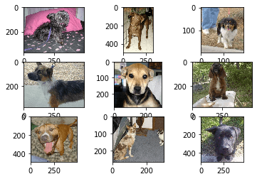
Kiểm tra lại dữ liệu đã giải nén bằng cách in ra một số hình chó.
from matplotlib import pyplot
from matplotlib.image import imread
# Define location of dataset
folder = dataset_folder
# Plot first few images
for i in range(9):
    # Define subplot
    pyplot.subplot(330 + 1 + i)
    # Define filename
    filename = folder + 'dog.' + str(i) + '.jpg'
    # Load image pixels
    image = imread(filename)
    # Plot raw pixel data
    pyplot.imshow(image)
# Show the figure
pyplot.show()
Chia dữ liệu
Phần này sẽ tạo ra dữ mục dataset_dogs_vs_cats chứa toàn bộ dữ liệu cần dùng, và chia theo thư mục như dưới. Thư mục train sẽ chứa toàn bộ dữ liệu cho training, thư mục val chứa dữ liệu cho validation và thư mục test sẽ chứa dữ liệu cho testing. Dữ liệu được chia lần lượt theo tỷ lệ 60%, 20%, 20%.
dataset_dogs_vs_cats
├── train
│   ├── cats
│   └── dogs
├── val
│   ├── cats
│   └── dogs
└── test
    ├── cats
    └── dogs
from os import makedirs
from os import listdir
from shutil import copyfile
from random import seed
from random import random

# Create directories
dataset_home = 'dataset_dogs_vs_cats/'
subdirs = ['train/', 'val/', 'test/']
for subdir in subdirs:
    # Create label subdirectories
    labeldirs = ['dogs/', 'cats/']
    for labldir in labeldirs:
        newdir = dataset_home + subdir + labldir
        makedirs(newdir, exist_ok=True)

# Copy dataset into folders
dog_files = []
cat_files = []

# Define ratio of pictures to use for testing
# Copy training dataset images into subdirectories
src_directory = dataset_folder
for file in listdir(src_directory):
    if file.startswith('cat'):
        cat_files.append(file)
    elif file.startswith('dog'):
        dog_files.append(file)

def train_validate_test_split(data, train_percent=.6, validate_percent=.2, seed=None):
    np.random.seed(seed)
    perm = np.random.permutation(np.arange(len(data)))
    m = len(data)
    train_end = int(train_percent * m)
    validate_end = int(validate_percent * m) + train_end

    train = np.array(data)[perm[:train_end]].copy()
    validate = np.array(data)[perm[train_end:validate_end]].copy()
    test = np.array(data)[perm[validate_end:]].copy()
    return train, validate, test

train_cats, val_cats, test_cats = train_validate_test_split(cat_files, seed=42, train_percent=.6, validate_percent=.2)
train_dogs, val_dogs, test_dogs = train_validate_test_split(dog_files, seed=42, train_percent=.6, validate_percent=.2)

list(map(lambda file: copyfile(src_directory + '/' + file, dataset_home + 'train/cats/' + file), train_cats))
list(map(lambda file: copyfile(src_directory + '/' + file, dataset_home + 'train/dogs/' + file), train_dogs))
list(map(lambda file: copyfile(src_directory + '/' + file, dataset_home + 'val/cats/' + file), val_cats))
list(map(lambda file: copyfile(src_directory + '/' + file, dataset_home + 'val/dogs/' + file), val_dogs))
list(map(lambda file: copyfile(src_directory + '/' + file, dataset_home + 'test/cats/' + file), test_cats))
list(map(lambda file: copyfile(src_directory + '/' + file, dataset_home + 'test/dogs/' + file), test_dogs))

print("Done!")
Tạo các ImageDataGenerator
Ở Keras, chúng ta có ImageDataGenerator để thực hiện tiền xử lý dữ liệu, đồng thời cung cấp dữ liệu cho cả quá trình training và testing. Ở dữ liệu training, chúng ta sử dụng thêm width_shift_range=0.1, height_shift_range=0.1, horizontal_flip=True cho data augmentation. Việc này sẽ tạo thêm dữ liệu bằng cách dịch ảnh, và lật ảnh theo chiều ngang (ảnh chó, mèo vẫn sẽ là chó, mèo khi thực hiện lật theo chiều ngang, không ảnh hưởng đến ý nghĩa ảnh). Việc chỉnh batch size được thực hiện tại đây.
from tensorflow.keras.preprocessing.image import ImageDataGenerator
train_datagen = ImageDataGenerator(rescale=1.0/255.0,
    width_shift_range=0.1, height_shift_range=0.1, horizontal_flip=True)
val_datagen = ImageDataGenerator(rescale=1.0/255.0)
test_datagen = ImageDataGenerator(rescale=1.0/255.0)
# prepare iterators
train_it = train_datagen.flow_from_directory('dataset_dogs_vs_cats/train/',
    class_mode='binary', batch_size=20, target_size=(224, 224))
val_it = val_datagen.flow_from_directory('dataset_dogs_vs_cats/val/',
    class_mode='binary', batch_size=20, target_size=(224, 224))
test_it = test_datagen.flow_from_directory('dataset_dogs_vs_cats/test/',
    class_mode='binary', batch_size=20, target_size=(224, 224))
Found 15000 images belonging to 2 classes.
Found 5000 images belonging to 2 classes.
Found 5000 images belonging to 2 classes.
II. VGG16
Sau việc chuẩn bị dữ liệu, chúng ta thực hiện việc xây dựng mạng VGG16 từ đầu trên Keras và huấn luyện mô hình để phân loại chó mèo.
Mọi người có thể đọc paper của VGG tại đây.
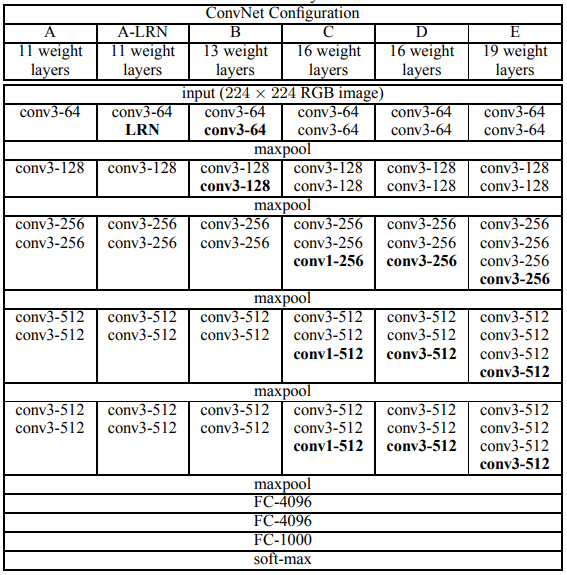
Hình ảnh kiến trúc VGG - https://arxiv.org/abs/1409.1556
Chúng ta sẽ tập trung vào hình ảnh kiến trúc mạng. Hình ảnh trên mô tả các kiến trúc mạng VGG, lấy từ paper. Chúng ta sẽ implement VGG16 (tức kiến trúc có 16 lớp (16 weight layers)). Tuy nhiên vì chúng ta chỉ phân loại 2 lớp (chó, mèo), sử dụng binary cross entropy làm loss function nên cần thay FC-1000 thành 1 lớp Fully Connected kích thước 1 và activation là sigmoid. Các bạn tham khảo phần mã nguồn bên dưới.
import tensorflow as tf
import tensorflow.keras
from tensorflow.keras.layers import Dense, Activation, Dropout, Flatten
from tensorflow.keras.layers import Conv2D
from tensorflow.keras.layers import MaxPooling2D

for gpu in tf.config.experimental.list_physical_devices('GPU'):
    tf.compat.v2.config.experimental.set_memory_growth(gpu, True)

model = Sequential()

model.add(Conv2D(64, (3,3), activation="relu", padding="same", kernel_initializer='he_uniform', name='block1_conv1', input_shape=(224, 224, 3)))
model.add(Conv2D(64, (3,3), activation="relu", padding="same", kernel_initializer='he_uniform', name='block1_conv2'))
model.add(MaxPooling2D(pool_size=(2,2), strides=(2,2), name='block1_maxpool'))

model.add(Conv2D(128, (3,3), activation="relu", padding="same", kernel_initializer='he_uniform', name='block2_conv1'))
model.add(Conv2D(128, (3,3), activation="relu", padding="same", kernel_initializer='he_uniform', name='block2_conv2'))
model.add(MaxPooling2D(pool_size=(2,2), strides=(2,2), name='block2_maxpool'))

model.add(Conv2D(256, (3,3), activation="relu", padding="same", kernel_initializer='he_uniform', name='block3_conv1'))
model.add(Conv2D(256, (3,3), activation="relu", padding="same", kernel_initializer='he_uniform', name='block3_conv2'))
model.add(Conv2D(256, (3,3), activation="relu", padding="same", kernel_initializer='he_uniform', name='block3_conv3'))
model.add(MaxPooling2D(pool_size=(2,2), strides=(2,2), name='block3_maxpool'))

model.add(Conv2D(512, (3,3), activation="relu", padding="same", kernel_initializer='he_uniform', name='block4_conv1'))
model.add(Conv2D(512, (3,3), activation="relu", padding="same", kernel_initializer='he_uniform', name='block4_conv2'))
model.add(Conv2D(512, (3,3), activation="relu", padding="same", kernel_initializer='he_uniform', name='block4_conv3'))
model.add(MaxPooling2D(pool_size=(2,2), strides=(2,2), name='block4_maxpool'))

model.add(Conv2D(512, (3,3), activation="relu", padding="same", kernel_initializer='he_uniform', name='block5_conv1'))
model.add(Conv2D(512, (3,3), activation="relu", padding="same", kernel_initializer='he_uniform', name='block5_conv2'))
model.add(Conv2D(512, (3,3), activation="relu", padding="same", kernel_initializer='he_uniform', name='block5_conv3'))
model.add(MaxPooling2D(pool_size=(2,2), strides=(2,2), name='block5_maxpool'))

model.add(Flatten())
model.add(Dense(4096, activation='relu'))
model.add(Dense(4096, activation='relu'))
model.add(Dense(1, activation='sigmoid'))

def optimizer_init_fn():
    learning_rate = 1e-4
    return tf.keras.optimizers.Adam(learning_rate)

model.compile(optimizer=optimizer_init_fn(),
              loss='binary_crossentropy',
              metrics=['accuracy'])

# Fit model (training)
history = model.fit_generator(train_it, steps_per_epoch=len(train_it),
    validation_data=val_it, validation_steps=len(val_it), epochs=50, verbose=1)
Epoch 1/20
750/750 [==============================] - 274s 365ms/step - loss: 0.6539 - accuracy: 0.6133 - val_loss: 0.5673 - val_accuracy: 0.7050
Epoch 2/20
750/750 [==============================] - 272s 362ms/step - loss: 0.5619 - accuracy: 0.7081 - val_loss: 0.5001 - val_accuracy: 0.7540
Epoch 3/20
750/750 [==============================] - 272s 362ms/step - loss: 0.4555 - accuracy: 0.7885 - val_loss: 0.4330 - val_accuracy: 0.7998
Epoch 4/20
750/750 [==============================] - 273s 363ms/step - loss: 0.3532 - accuracy: 0.8419 - val_loss: 0.3022 - val_accuracy: 0.8756
Epoch 5/20
750/750 [==============================] - 273s 364ms/step - loss: 0.2720 - accuracy: 0.8849 - val_loss: 0.2449 - val_accuracy: 0.8976
Epoch 6/20
750/750 [==============================] - 274s 365ms/step - loss: 0.2193 - accuracy: 0.9089 - val_loss: 0.2297 - val_accuracy: 0.9058
Epoch 7/20
750/750 [==============================] - 273s 363ms/step - loss: 0.1929 - accuracy: 0.9210 - val_loss: 0.2055 - val_accuracy: 0.9112
Epoch 8/20
750/750 [==============================] - 272s 363ms/step - loss: 0.1651 - accuracy: 0.9317 - val_loss: 0.2105 - val_accuracy: 0.9174
Epoch 9/20
750/750 [==============================] - 275s 367ms/step - loss: 0.1487 - accuracy: 0.9402 - val_loss: 0.1920 - val_accuracy: 0.9192
Epoch 10/20
750/750 [==============================] - 272s 362ms/step - loss: 0.1421 - accuracy: 0.9423 - val_loss: 0.1536 - val_accuracy: 0.9370
Epoch 11/20
750/750 [==============================] - 271s 361ms/step - loss: 0.1211 - accuracy: 0.9508 - val_loss: 0.1670 - val_accuracy: 0.9334
Epoch 12/20
750/750 [==============================] - 270s 361ms/step - loss: 0.1151 - accuracy: 0.9533 - val_loss: 0.1756 - val_accuracy: 0.9322
Epoch 13/20
750/750 [==============================] - 270s 360ms/step - loss: 0.1077 - accuracy: 0.9581 - val_loss: 0.1545 - val_accuracy: 0.9398
Epoch 14/20
750/750 [==============================] - 271s 361ms/step - loss: 0.0991 - accuracy: 0.9605 - val_loss: 0.1451 - val_accuracy: 0.9418
Epoch 15/20
750/750 [==============================] - 270s 361ms/step - loss: 0.0908 - accuracy: 0.9640 - val_loss: 0.1666 - val_accuracy: 0.9382
Epoch 16/20
750/750 [==============================] - 271s 361ms/step - loss: 0.0861 - accuracy: 0.9647 - val_loss: 0.1828 - val_accuracy: 0.9374
Epoch 17/20
750/750 [==============================] - 270s 360ms/step - loss: 0.0831 - accuracy: 0.9689 - val_loss: 0.1423 - val_accuracy: 0.9406
Epoch 18/20
750/750 [==============================] - 270s 361ms/step - loss: 0.0726 - accuracy: 0.9713 - val_loss: 0.1512 - val_accuracy: 0.9404
Epoch 19/20
750/750 [==============================] - 271s 361ms/step - loss: 0.0693 - accuracy: 0.9716 - val_loss: 0.1506 - val_accuracy: 0.9454
Epoch 20/20
750/750 [==============================] - 272s 362ms/step - loss: 0.0695 - accuracy: 0.9732 - val_loss: 0.1505 - val_accuracy: 0.9496
Kết quả
Ở bước này, chúng ta visualize lại toàn bộ quá trình training, đồng thời test model trên tập testing (20% chia ra từ bộ dữ liệu ban đầu). Sau khi nhận được đồ thị visualize quá trình training, chúng ta có thể sử dụng để tinh chỉnh các tham số như batch size, learning rate bằng cách quay lại các bước trên.
# Baseline model with data augmentation for the dogs vs cats dataset
import sys
from matplotlib import pyplot as plt

# Plot diagnostic learning curves
def summarize_diagnostics(history):

    plt.plot(history.history['accuracy'])
    plt.plot(history.history['val_accuracy'])
    plt.title('model accuracy')
    plt.ylabel('accuracy')
    plt.xlabel('epoch')
    plt.legend(['train', 'val'], loc='upper left')
    plt.show()

    plt.plot(history.history['loss'])
    plt.plot(history.history['val_loss'])
    plt.title('model loss')
    plt.ylabel('loss')
    plt.xlabel('epoch')
    plt.legend(['train', 'val'], loc='upper left')
    plt.show()

# Evaluate model
_, acc = model.evaluate_generator(test_it, steps=len(test_it), verbose=1)
print('> %.3f' % (acc * 100.0))

# Learning curves
summarize_diagnostics(history)
250/250 [==============================] - 25s 99ms/step - loss: 0.1411 - accuracy: 0.9534
95.340
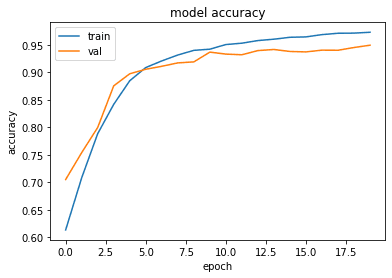
Vậy là chúng ta đã có thể code lại VGG16 và áp dụng phân loại chó mèo với độ chính xác lên đến 95.34 % !! Các bạn có thể áp dụng thêm các kỹ thuật khác như thêm một số layer Dropout để tăng độ chính xác và giảm overfiting cho mô hình.
Mọi góp ý cho bài viết các bạn hãy viết ở dưới comment nhé. Xin cảm ơn!