[MOOC] Apollo Lesson 6: Planning

My note for lesson 6 of MOOC course: Self-Driving Fundamentals - Featuring Apollo. Content: Identify several different approaches Apollo uses to develop trajectories for autonomous vehicles.

In planning, we incorporate HP maps, localization and prediction to build a trajectory for the vehicle. The first step is route navigation, which focuses on how to go from A to B on the map. This step is like the navigation app on your phone. After route planning, we zoom into trajectory planning, which make subtle decisions to avoid obstacles and create a smooth ride for passengers.

Routing

Routing is to find the best path from A to B on a map.

Inputs:

The map: Apollo provides map data, including the road network and realtime traffic information.
Our current position on the map
Our destination

Output: The route to the destination.

World to Graph

Apollo uses graph to represent the map.

Nodes: Sections of road
Edges: Connections between those sections

Map → Map Graph → Best Route on Graph → Best Route on Map

We can use A* algorithm to search on the graph.

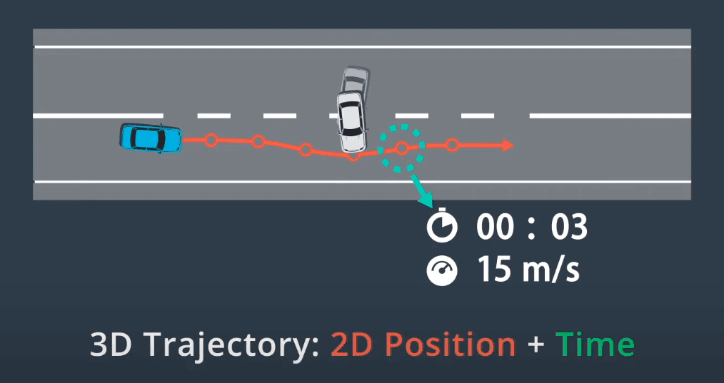
3D trajectory

3D trajectory is made of 2D position (waypoint) and time.

Real-world planning faces multiple constraints:

The trajectory should be collision-free
We want passengers to feel comfortable
The trajectory should be physically viable for the vehicle

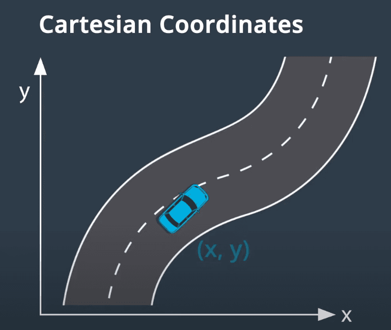
Frenet coordinates

Cartesian coordinates aren't optimal for a vehicle because it's hard to know how far the car has traveled or whether it's deviated from the center of the lane.

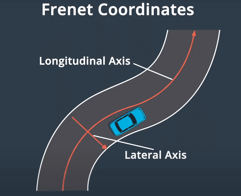
Therefore, we need Frenet coordinates, which describe the position of a car with respect to the road. Frenet has 2 axes: longitudinal axis and lateral axis.

Path-velocity decoupled planning

Trajectory Planning = Path Planning + Speed Planning

Path Planning: Generate candidate curves. Rank each path by smoothness, safety, deviation from the lane center, .. and select the best path.
Speed Planning: Determine what speed of vehicle in each waypoint. → Speed profiler.

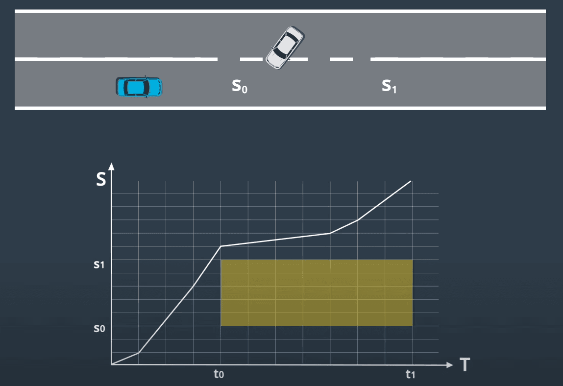
ST graph

ST graph is a tool which can help us design and select the speed profile. In an ST graph, S represents the longitudinal displacement of the vehicle and T represents time.

In order to build the best speed profile, we discretize the ST graph into multiple cells. Suppose the prediction module predicts that a car will cut into our lane from time t0 to t1. Since the car will occupy positions S0 to S1 during that time period, we draw a yellow rectangle to block this area on ST graph. In order to avoid a collision, our speed profile must not intersect this rectangle.

In real-world situations, many constraints can affect the optimization process for speed profile, such as speed limit, physical properties of the car, and the obstacles.

Optimization

From discrete solution, we use quadratic programming to generate a smooth speed profile.

End-to-end example

Suppose we are control a car to avoid an obstacle.

Generate candidate paths → Evaluate paths using a cost function → Select the lowest cost path → Use ST graph to create speed profile → Use quadratic programming to smooth the path and speed profile → Bind results to construct a trajectory.

Lattice programming

Lattice programming is a trajectory generation approach using Frenet coordinates. We decompose 3D problem into different 2D problems: 3D trajectory → the longitudinal trajectory with timestamps (ST trajectory) + the lateral offset relative to the longitudinal trajectory (SL trajectory).

Step 1: Project our environment onto a longitudinal axis and a lateral axis and develop the ST and SL trajectory independently.
Step 2: Combine the results.

Source of Lattice programming in Apollo: https://github.com/ApolloAuto/apollo/blob/master/modules/planning/planner/lattice/lattice_planner.cc.